AFAM 188: R 6 R Assignment 2
Please add your name and email to the below lines:
Name:
Email:
6.1 Instructions
Complete the R coding challenges and questions in RStudio Cloud Project <> in the r-assignment-2.R file. Save that file as you work. You will have until 12/06 by 5pm. If you encounter any problems, please come to
office hours on 12/3 from 2-4pm in the Data Science Center, 21536 YRL, email us at datascience@ucla.edu or set up an appointment.
This assignment is worth 32 points.
6.2 1. For this exercise we need to load packages in R. (3 points)
6.3 2. We also will need to load the data we will be using to map in R. Load the data. (3 points)
arrests <- read_csv('data/aug6_12_arrest_data.csv')
arrests_sf <- st_as_sf(arrests, coords = c("longitude", "latitude"), crs = 4326)
#geometry type:  MULTILINESTRING
la_county <- st_read(dsn ="data/DRP_COUNTY_BOUNDARY/DRP_COUNTY_BOUNDARY.shp")
## Reading layer `DRP_COUNTY_BOUNDARY' from data source `/Users/timdennis/instruction/afam188/afam188-r/data/DRP_COUNTY_BOUNDARY/DRP_COUNTY_BOUNDARY.shp' using driver `ESRI Shapefile'
## Simple feature collection with 2 features and 2 fields
## geometry type: MULTILINESTRING
## dimension: XY
## bbox: xmin: 6280000 ymin: 1380000 xmax: 6670000 ymax: 2120000
## epsg (SRID): 2229
## proj4string: +proj=lcc +lat_1=35.46666666666667 +lat_2=34.03333333333333 +lat_0=33.5 +lon_0=-118 +x_0=2000000.0001016 +y_0=500000.0001016001 +ellps=GRS80 +towgs84=0,0,0,0,0,0,0 +units=us-ft +no_defs## Reading layer `Los_Angeles_City_Zip_Codes' from data source `/Users/timdennis/instruction/afam188/afam188-r/data/Los_Angeles_City_Zip_Codes/Los_Angeles_City_Zip_Codes.shp' using driver `ESRI Shapefile'
## Simple feature collection with 157 features and 7 fields
## geometry type: MULTIPOLYGON
## dimension: XY
## bbox: xmin: -119 ymin: 33.7 xmax: -118 ymax: 34.3
## epsg (SRID): 4326
## proj4string: +proj=longlat +datum=WGS84 +no_defs#geometry type: MULTILINESTRING
## the below command will make our zip data valid
la_zips <- lwgeom::st_make_valid(la_zips)
la_freeways <- st_read(dsn ="data/CAMS_FREEWAY_SHIELDS/CAMS_FREEWAY_SHIELDS.shp")## Reading layer `CAMS_FREEWAY_SHIELDS' from data source `/Users/timdennis/instruction/afam188/afam188-r/data/CAMS_FREEWAY_SHIELDS/CAMS_FREEWAY_SHIELDS.shp' using driver `ESRI Shapefile'
## Simple feature collection with 45 features and 4 fields
## geometry type: MULTILINESTRING
## dimension: XY
## bbox: xmin: 6280000 ymin: 1720000 xmax: 6670000 ymax: 2120000
## epsg (SRID): 2229
## proj4string: +proj=lcc +lat_1=35.46666666666667 +lat_2=34.03333333333333 +lat_0=33.5 +lon_0=-118 +x_0=2000000.0001016 +y_0=500000.0001016001 +ellps=GRS80 +towgs84=0,0,0,0,0,0,0 +units=us-ft +no_defs6.4 3. Altering a bubble map. (6pts)
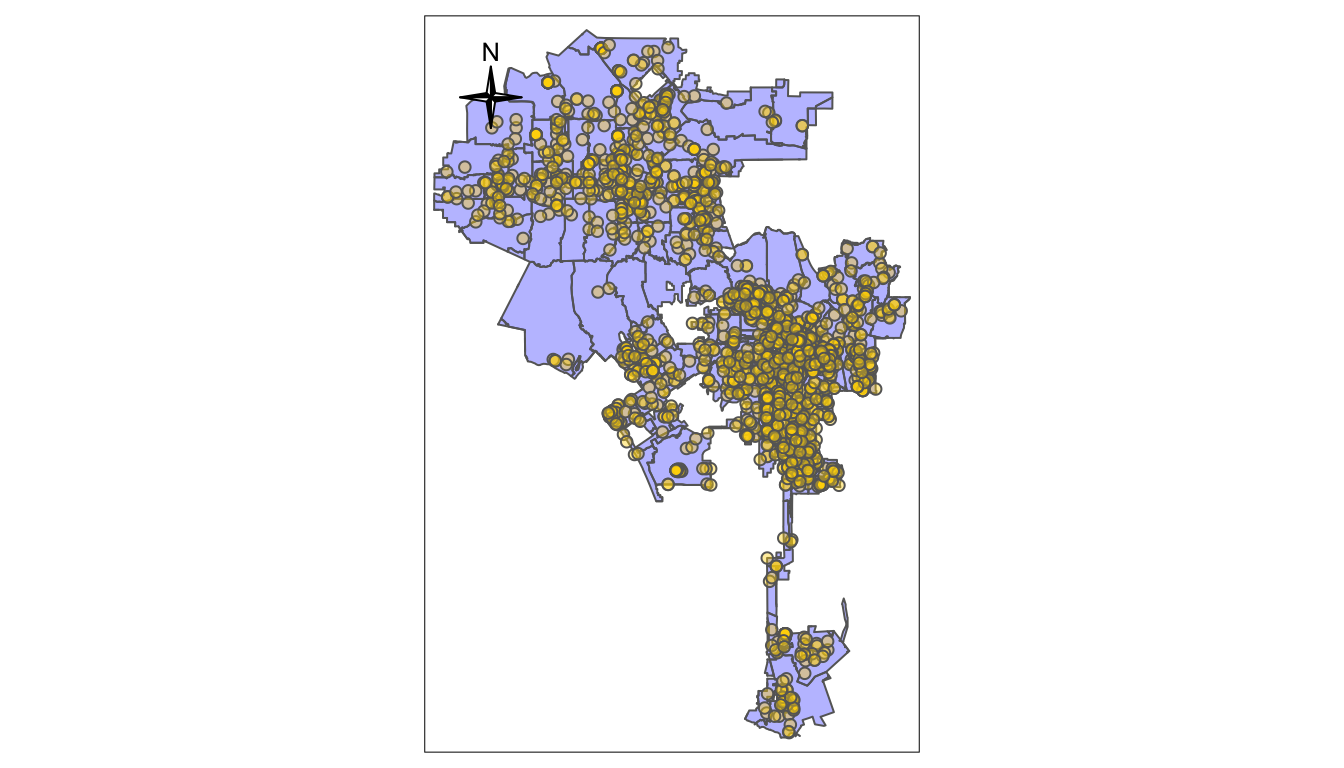
In class we made the below map using tmap.
tm_shape(la_zips) +
   tm_polygons(col="blue", alpha = 0.3) +
   tm_shape(arrests_sf) +
   tm_bubbles(size = 0.09, col="gold", alpha=0.4)+
tm_compass(type = "4star", position = c("left", "top"), size = 2) 
Alter the below code by filling in the blanks with a different color for the tm_polygons and tm_bubbles functions. Also, adjust the alpha parameters. What colors are available for you to use? You can run the below function colors() for a list:
6.5 4. Mapping arrests by sex (6pts)
Changing the map above so the bubbles are colored based on the sex variable in our data.
tm_shape(la_zips) +
   tm_polygons(col="blue", alpha = 0.3) +
   tm_shape(arrests_sf) +
   tm_bubbles(size = 0.09, col="___", palette=c(F='cyan', M='red')) +
   tm_compass(type = "4star", position = c("left", "top"), size = 2)
What does the map tell you about the data? Answer:
6.6 5. Using arrange to make a row of maps (7 points)
With the below code, we create multiple maps based off the base map lazips. Run the code, to create the R objects.
lazips <- tm_shape(la_zips)
lzip1 <- lazips + tm_fill(col = "red")
lzip2 <- lazips + tm_fill(col = "red", alpha = 0.3)
lzip3 <- lazips + tm_borders(col = "blue")
lzip4 <- lazips + tm_borders(lwd = 3)
Now, use the function tmap_arrange() to arrange lzip1 to lzip4, printing them out in a row of maps on the right plot. To see how we did this in class, see section 5.2 of the lesson: https://afam188.netlify.com/mapping-with-r-continued.html#saving-map-objects-1
6.7 6. Creating a faceted map (7 points)
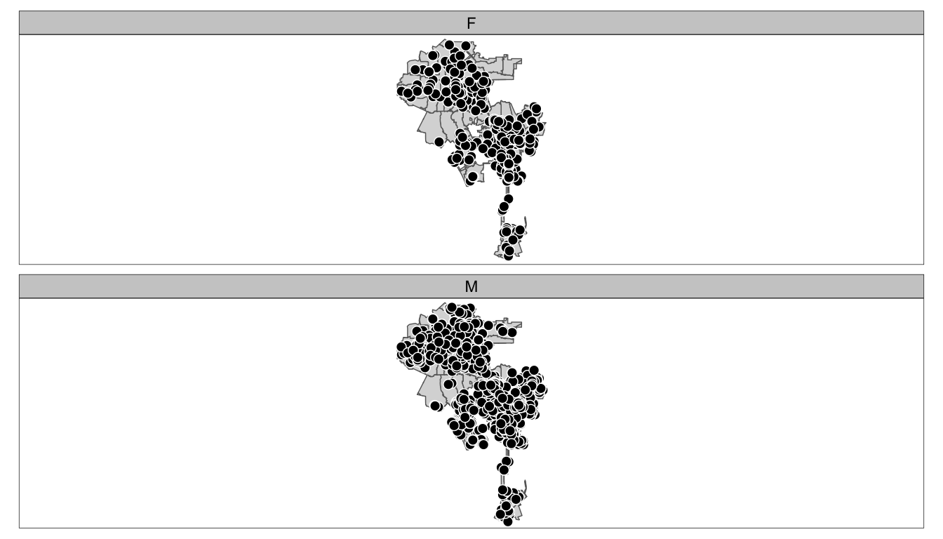
In class we produced a faceted map of arrests by sex with the below code. Run the code to see how it works:
tm_shape(la_zips) +
   tm_polygons() +
   tm_shape(arrests_sf) +
   tm_symbols(col = "black", border.col = "white", size = 0.5) +
   tm_facets(by = "sex", nrow=2, free.coords = FALSE)
Now, for below, fill in the blank in the tm_facets function to produce a faceted map of arrests by race category race_cat. This should produce a plot for each race category with arrest points colored by race.